Fiducio / paper
TMLR Transactions on Machine Learning Research · 2026

Rethinking Post-Hoc Calibration in Semantic Segmentation

Tristan Kirscher1,2,★, Kim-Celine Kahl3,4, Balint Kovacs3,5, Maximilian Rokuss3,4, Klaus Maier-Hein3,6, Xavier Coubez1,2, Philippe Meyer1,2, Sylvain Faisan1

  1. 1ICube Laboratory, CNRS UMR 7357, University of Strasbourg, France
  2. 2CLCC Institut Strauss, Strasbourg, France
  3. 3German Cancer Research Center (DKFZ), Division of Medical Image Computing, Heidelberg, Germany
  4. 4Faculty of Mathematics and Computer Science, University of Heidelberg, Germany
  5. 5Medical Faculty Heidelberg, Heidelberg University, Germany
  6. 6Pattern Analysis and Learning Group, Dept. of Radiation Oncology, Heidelberg University Hospital, Germany

★ Corresponding author: tristan.kirscher@unistra.fr

pip install fiducio
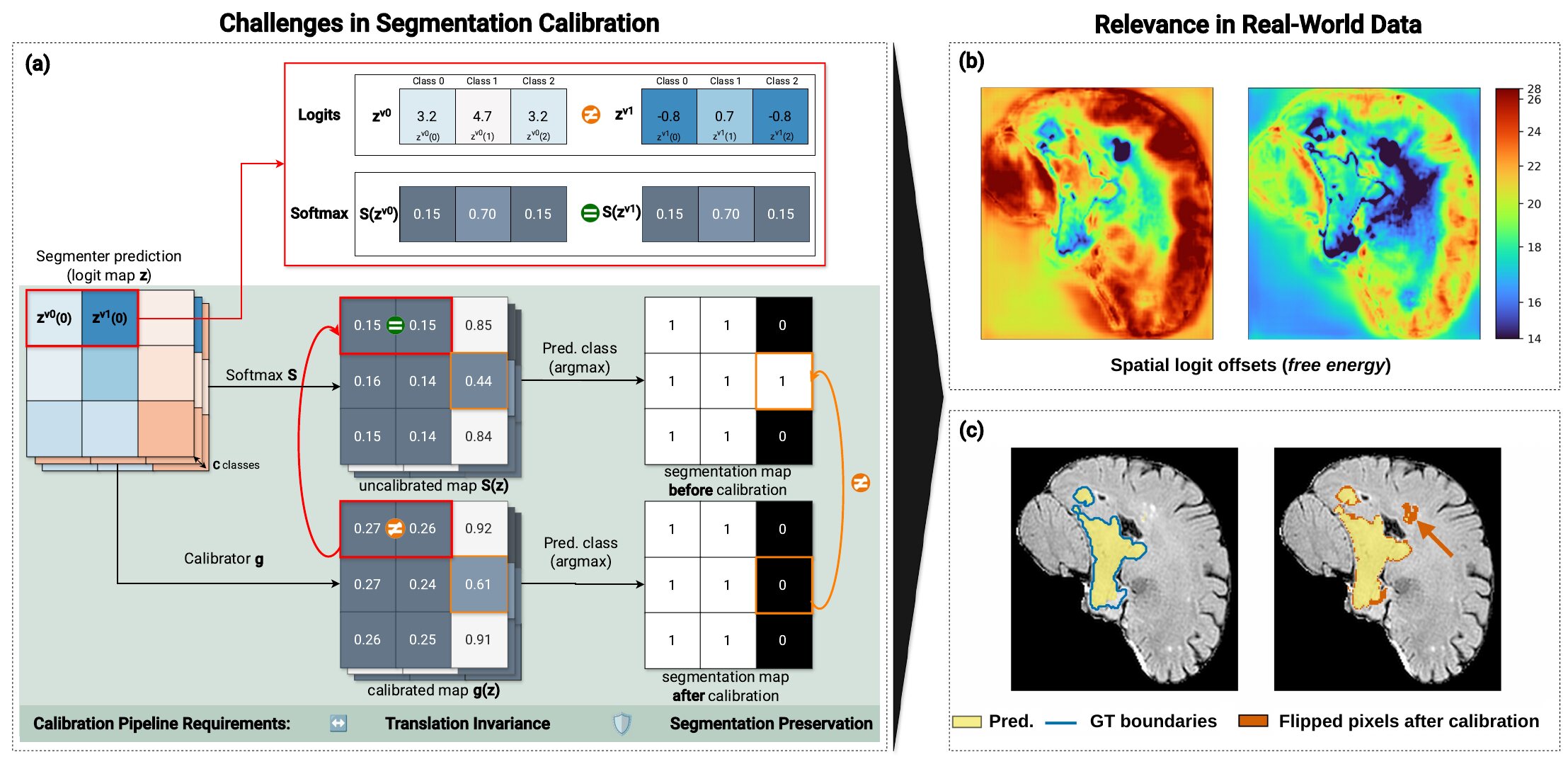
Figure 1 of the paper: (a) logits that differ by a constant give the same softmax, yet a calibrator can return different outputs, and calibration can flip the argmax; (b) spatial maps of logit free energy for two segmenters; (c) a brain-tumour example where calibration flips pixels at the tumour boundary.
Figure 1 of the paper. (a) Logits that differ only by a constant give the same softmax, yet a calibrator may return different outputs; calibration can also flip the argmax. (b) The additive logit component (free energy) varies across locations in real segmentation outputs. (c) Real BraTS example where calibration-induced flips perturb tumour boundaries.

01 · The problem in 30 seconds

Two structural issues calibration inherits from classification

Post-hoc calibration fits a small map on a held-out set and applies it to every pixel or voxel. In dense prediction, two overlooked properties of that map decide whether it is well defined and whether it leaves the segmentation alone.

Issue 1 · offset dependence

Same probabilities, different calibrated output

Adding a constant to all logits of a pixel leaves the softmax unchanged, but several standard calibrators still depend on that arbitrary offset. In segmentation the offset varies across pixels.

S(z + c·1) = S(z)  but  g(z + c·1) ≠ g(z)
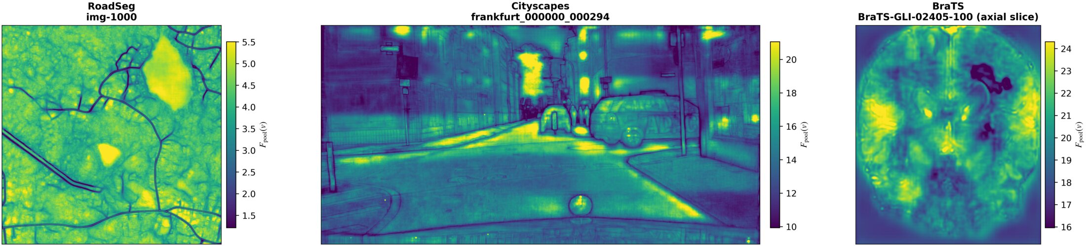
Spatial maps of pooled-logit free energy for a RoadSeg, a Cityscapes and a BraTS test image; the offset varies strongly across each image.
Pooled-logit free energy Fpool(v) = log Σc exp zpool,c(v) on test images (paper Fig. 3).

Spatial std of the offset per image (logit units)

Mean over held-out cases of Stdv(Fpool(v)), whiskers = interquartile range, 5-model nnU-Net ensembles (paper Table 3). It shows the offset is present, not how much a non-TI calibrator loses.
Issue 2 · loss mismatch

Calibration can rewrite the segmentation

Segmenters are trained with soft Dice + cross-entropy; the calibrator is fitted with cross-entropy on a small held-out set (50 cases here). An unconstrained calibrator can then change the argmax and lower Dice.

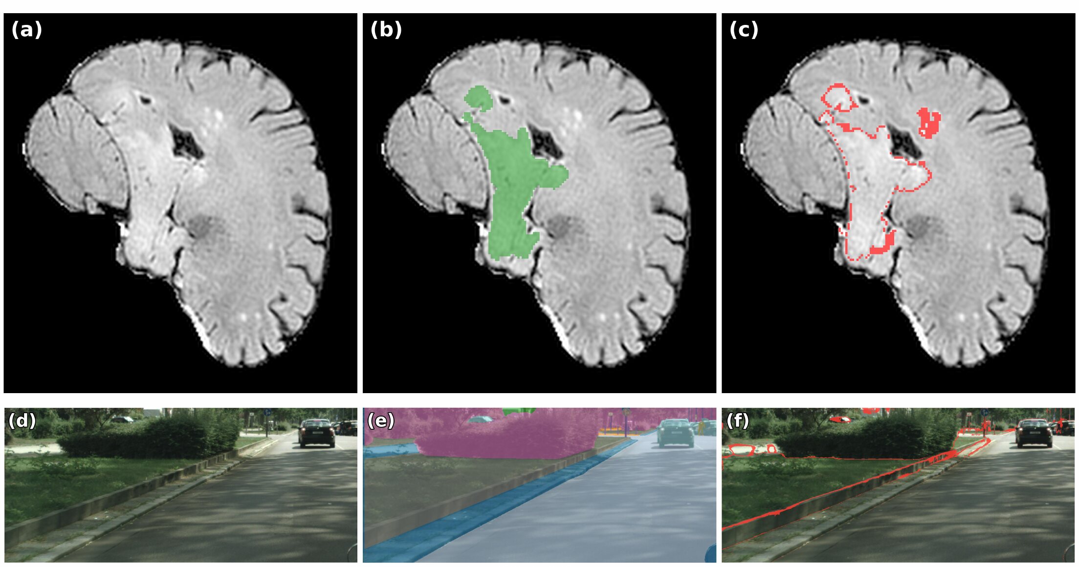
BraTS and Cityscapes examples: input, ground truth, and in red the pixels whose label flips after matrix scaling; flips concentrate at boundaries.
Pixels flipped by MS(z̄), in red: they concentrate near tumour and semantic boundaries (paper Fig. 4, App. D).

Flip audit of MS(z̄)

Share of flipped pixels that turn a correct prediction wrong (harmful) or a wrong one correct (beneficial); the remainder leaves voxel accuracy unchanged (paper §4.3).

02 · Key insights

Two constraints that make calibration well defined

Each constraint gets a matched counterpart, so its effect can be measured on its own. Try the two toy demos: they run the actual constructions from the paper on hand-picked numbers.

Insight 1 · translation invariance (TI) toy · 3 classes
g(z) = g(z + c·1)  ∀ z, c

TS, ETS and DC are TI. MS is TI iff all rows of W have the same sum, so MSc enforces that constraint; feeding log S(z) = z − F(z)·1 instead of z also makes a calibrator TI (DC, LTS(log S)).

+0.0

Weights chosen by hand for illustration, not fitted. With row sums W·1 = (1.5, 1.1, 0.7), MS drifts with c and, as c → +∞, collapses onto class k* = argmax(W·1) whatever S(z) is (paper §3.1). MSc uses W·1 = 1.1·1.

Insight 2 · decision preservation toy · 48×30 map
argmax g(z) = argmax z  (CMSap)  ·  order kept (CMSop)

Forcing VS or MS to preserve the argmax collapses them to temperature scaling. Class-conditional maps avoid this: one affine expert per predicted class, each constrained to keep the argmax (or order) cone invariant.

0.80
segmentation after · ■ flipped
confidence after (max q)

Toy logits with small margins near region boundaries. The argmax-preserving map is the paper's parameterisation W = G⁻¹W′G with non-negative block A and bias in the cone; confidence still moves, labels cannot. Expert parameters grow as O(C³), so CDC/CMS suit low-to-moderate class counts.

03 · Results

Matched comparisons on three benchmarks

Five-model nnU-Net ensembles, calibrators fitted on 50 held-out cases, 3 random repeats. A difference counts as significant when its 95% paired hierarchical-bootstrap interval excludes zero (paper criterion).

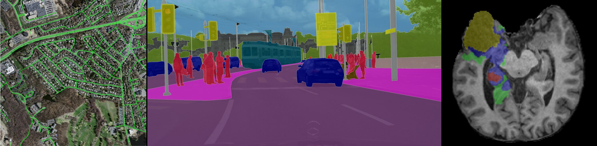
Sample inputs with ground-truth overlays from Massachusetts Roads, Cityscapes and BraTS 2024.
RoadSeg (Massachusetts Roads, 2D aerial, C = 2) · Cityscapes (2D urban, C = 20) · BraTS GLI 2024 (3D MRI, C = 5; one slice shown). Paper Fig. 2.

What the paper concludes, at its significance level

ComparisonRoadSeg · C=2BraTS · C=5Cityscapes · C=20
TI, affineMS(z̄) → MSc, DC DC significantly better on NLL, ECE, BA-ECE
MSc too restrictive for C = 2: significantly worse BA-ECE
Improvements not significant Both significantly better on NLL, ECE, BA-ECE (ACE not testable). NLL 0.404 → 0.324–0.328
TI, localLTS(z̄) → LTS(log S(z̄)) ECE 0.004 → 0.002, significant; other metrics not Lower on most metrics, not significant Not significant; BA-ECE unchanged
Decision preservationCDC → CMSap, CMSop Pooled DSC kept: 76.7 vs 75.7 for CDC
Clear calibration cost: CDC better on all metrics, significant in most cases
DSC preserved; BA-ECE significantly better in 4/4 comparisons; NLL/ECE close; ACE mixed DSC preserved; BA-ECE significantly better in 4/4, NLL in 3/4; ECE slightly up or unchanged

significant in favour of the constraint   significant against / cost   not significant. Summarised from §4.3 and Appendix I (Tables 9–10) of the paper.

Paired differences with 95% CIs

Hover or focus an interval for its values.
CI excludes 0, favours the constrained method CI excludes 0, against it not significant

Constrained minus reference, from paper Tables 9–10 (App. I). Each panel has its own axis. ACE and flip rate are not paired endpoints, so the paper gives them no test.

Decision preservation keeps the pooled Dice

DSC (%) with 95% CIs. CMSap and CMSop keep the pooled segmentation by construction; CDC does not.

CDC (unconstrained)CMSap / CMSop

TI alone does not prevent flips: MS, MSc and DC on z̄ drop Cityscapes DSC from 79.4 to 70.4–73.4 and BraTS from 76.9 to 67.6–70.2.

Practical takeaways (paper §4.3, point 4)

  • Translation invariance is a structural requirement and, in the matched comparisons, an empirically beneficial constraint: recommended by default.
  • Decision preservation is mandatory when the deployed segmentation must not change. Otherwise it reduces capacity with a dataset-dependent effect: compare constrained and unconstrained calibrators on a selection split held out from the fitting data.
  • No single calibrator is best across datasets and metrics. The in-distribution trends persist under corruption-based covariate shift on Cityscapes (Appendix H).

Reliability, uncalibrated vs best calibrated

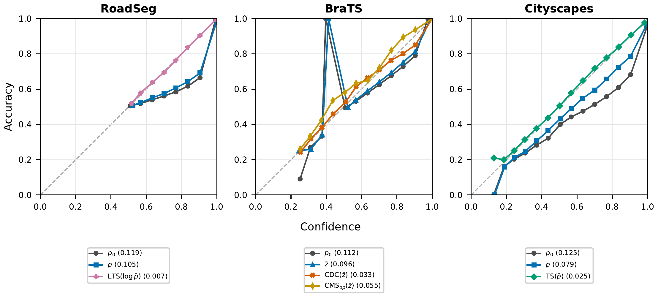
Reliability diagrams for RoadSeg, BraTS and Cityscapes comparing the single model, the pooled ensemble and the best-ACE calibrated methods.
Test-split reliability curves; numbers in parentheses are mean test ACE. For each dataset, the best-ACE calibrated method overall and the best-ACE order-preserving one (paper Fig. 8, App. J).

04 · Quickstart

Calibrate any segmenter's logits

Fiducio only sees (B, C, *spatial) tensors, so it works with any 2D or 3D model. Core dependencies: numpy and torch.

import torch
from fiducio import TemperatureScaling, load_calibrator

# From a held-out, labelled calibration set:
logits = torch.randn(8, 4, 64, 64)          # (B, C, H, W) model logits
labels = torch.randint(0, 4, (8, 64, 64))   # (B, H, W) labels

calibrator = TemperatureScaling(input_type="logits").fit(logits, labels)

# Apply to new predictions (returns calibrated probabilities):
probs = calibrator.transform(torch.randn(2, 4, 64, 64))

# Save and reload (loads on CPU by default):
calibrator.save("calibrator.pt")
calibrator = load_calibrator("calibrator.pt")

Paper method → class

Same fit / transform API for every calibrator.

PaperClassTIKeeps
TSTemperatureScalingyesorder
MSMatrixScalingno—
MScTranslationInvariantMatrixScalingyes—
DCDirichletCalibrationyes—
CDCClassConditionalMatrixScalingyes—
CMSapArgmaxPreservingMatrixScalingyesargmax
CMSopOrderPreservingMatrixScalingyesorder

From the Fiducio README. Full guide: quickstart · calibrators.

05 · Citation

BibTeX

@article{kirscher2026rethinking,
  title   = {Rethinking Post-Hoc Calibration in Semantic Segmentation},
  author  = {Kirscher, Tristan and Kahl, Kim-Celine and Kovacs, Balint and
             Rokuss, Maximilian and Maier-Hein, Klaus and Coubez, Xavier and
             Meyer, Philippe and Faisan, Sylvain},
  journal = {Transactions on Machine Learning Research},
  issn    = {2835-8856},
  year    = {2026},
  url     = {https://openreview.net/forum?id=xwNoSNxgxV}
}